▷ How to Create Pivot Tables in Excel
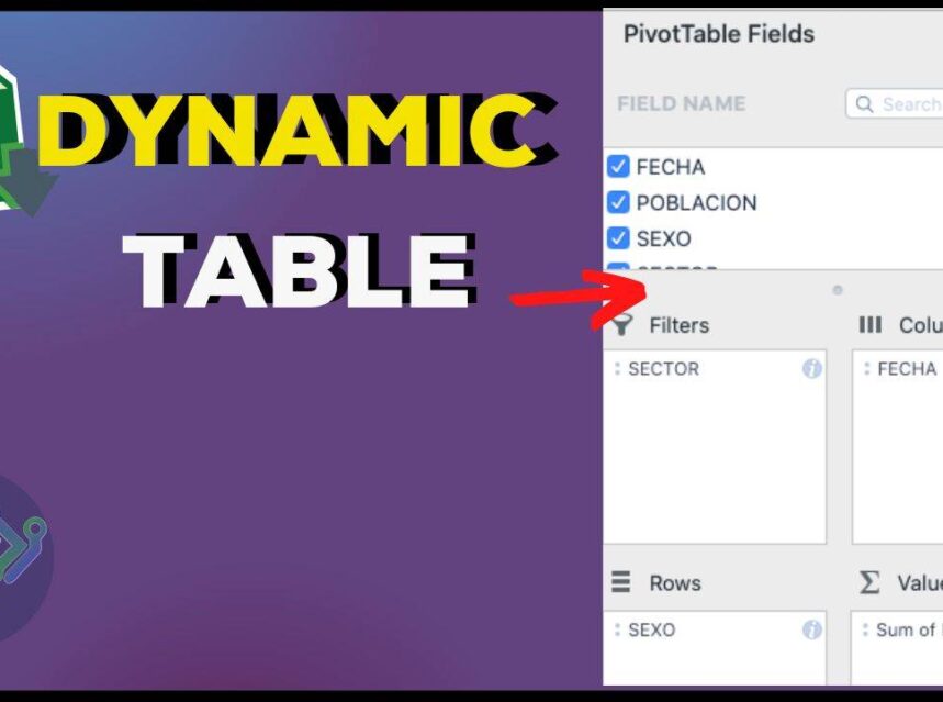
To create pivot tables in excel es importante conocer que esta es una herramienta de excel muy utilizada para organizar, resumir, agrupar y analizar la información de forma rápida y sencilla, desde las opciones que brinda de la lista de campos de la tabla dinámicas para organizar como: filters, columns, rows, values.
When you have a very large amount of information in excel, spread over several columns and/or rows, data that is repeated and you want to simplify the information, you can use pivot tables, even generate graphs with the results of the report.
They can also customize the display of the information, changing the font, size, layout of the pivot table and use other options such as "analyze pivot table" to create graphs.
The information fields, which are the titles of the information contained in the columns, are organized in the following areas in order to create the pivot tables:
AREAS OF THE PIVOT TABLE:
- FILTERS: This area contains the information that you want to display in the pivot table and also the information that is excluded.
- COLUMNS: Contains the table headings horizontally.
- ROWS: Contains the information that appears in the cells vertically.
- VALORES: Datos que sean agregados o llevan algún calculo.
To create a pivot table, you must have a base information in an excel sheet, this can be contained in a table or not, it must be coherent according to the organization in cells and columns so that at the moment of organizing it in the pivot table it is much simpler.
In this case, we will use as an example the information on the population in Colombia from 2014 to 2021:

As we can see, the information contained in the date column, gender (Female/Male) and sector (North, South, East), is repeated to such an extent that at first glance we cannot analyze, for example, the amount of population over the years, or according to the sector of Colombia, how many men or women there are, etc. With the dynamic table we can analyze the information extensively and conclude your own observations.
The excel template containing the developed pivot table can be downloaded from the following link:
DOWNLOAD - DYNAMIC TABLE EXERCISE ENGLISH
RELATED POST:
- Data validation in excel
- Convert text to columns
- Dynamic tables
- Excel templates with pivot table examples
Steps to create pivot tables in excel:
- Select all the information that will be included in the pivot table:

2. Ir al menu de herramientas > Insertar > Tablas> Tabla dinámica > aparece una ventana de configuración:

3. En la ventana de configuración puedes select a table or range (in this case in step 1 we have already selected the information) or you can use an external data source.
4. Seleccionar dónde desea ubicar la tabla dinámica, puede ser en una New spreadsheet inside the book you are using or in a Existing spreadsheet > accept.

5. Select the fields of the list of pivot table fields and arrange in the boxes. In this case we will organize the information by dragging the fields between the areas as follows:

The pivot table will be displayed on the right side like this:

Other Tips when inserting pivot tables:
You can organize the information in any way you wish to discover different ways of analyzing the information contained in the pivot table, for example:
By adding the Sector in the area of FILTERSYou can filter the information to know the population according to the sector of Colombia (North, South, East) and separated by gender (Male/Female) over the years.

Like this previous example, you can organize the information to obtain the results you want, depending on the purpose of the pivot table.
6. To change the design of the pivot table, two new tools are generated in the upper part: automate and Acrobat, according to the excel select the following symbol >> Here, two options are displayed, select Design.

Here you can discover tools such as: subtotals, Grand totals, Report layout, Blank rows, You can also select how you want the colors to be displayed in the table and choose the color and layout of the table.

If you want to change the font style, color, size, modify the number format of the values, you can select the cells to be modified and do it with the tool Home, pues no hay limitaciones de las otras herramientas al crear tablas dinámicas.
VIDEO: COMO INSERTAR TABLA DINÁMICA PASO A PASO


